Maximum Likelihood Estimation via Maximum-Likelihood

using Flux, ForwardDiff, Distributions, Plots, StatsPlots, Random, Zygote, LinearAlgebra, ChainRules, ChainRulesCore

Simple latent variable model

\[X\sim\mathcal{N}(\mu_h,\sigma_h^2)\] \[Y\sim\mathcal{N}(\exp(\alpha_o\cdot X),\sigma_o^2)\]

struct LatentModel
    mu_h
    sigma_h
    alpha_o
    sigma_o
end
Flux.@functor LatentModel

LatentModel() = LatentModel(zeros(1,1),zeros(1,1),ones(1,1),zeros(1,1))

function Base.rand(m::LatentModel, N::Int)
    mu_h = m.mu_h[1]
    sigma_h = exp(m.sigma_h[1])
    
    alpha_o = m.alpha_o[1]
    sigma_o = exp(m.sigma_o[1])
    
    X = randn(N) .* sigma_h .+ mu_h
    Y = randn(N) .* sigma_o .+ exp.(alpha_o.*X)
    
    return Y
end

Base.rand(m::LatentModel) = rand(m,1)[1]

Specify model for a test case

\[X\sim\mathcal{N}(1,0.25)\] \[Y\sim\mathcal{N}(\exp(0.75\cdot X),0.25)\]

Random.seed!(123)

true_model = LatentModel([1.0], [log(0.5)], [0.75], [log(0.5)])

Yfull = rand(true_model,50000) #to plot the density
Y = Yfull[1:150]

histogram(Y,bins=20,normalize=true,alpha=0.5,label="Data",fmt=:png)
density!(Yfull,c=:red,lw=2, label="True density (apprx.)")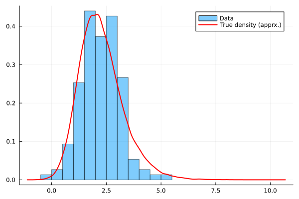

True density

\[p_\theta(y)=\int p_\theta(y|x)\frac{p_\theta(x)}{q(x)} q(x)dx\]

Approximated density

\[\hat{p}_\theta(y)=\frac{1}{M}\sum_{j=1}^M p_\theta(y|x_j)\frac{p_\theta(x_j)}{q(x_j)}\]

with \(x_j\) the proposal sample, drawn from \(q(x)\) with sample size \(M\).

Here:

\[q(x)=\mathcal{N}(x|0,4)\]

function particle_ll(m::LatentModel, y, M=1000)
    N = length(y)
    
    qdist = Normal(0,2) #q(x))
    pdist = Normal(m.mu_h[1],exp(m.sigma_h[1])) #p(x)
    
    ps = map(_->rand(qdist,M), 1:N)
    
    #one particle sample (1:M) per observation (1:N)
    odists = map(i->Normal.(exp.(m.alpha_o[1].*ps[i]),exp(m.sigma_o[1])),1:N)
    
    #p(y_i) = 1/M sum_j^M[p(y_i|x_j)p(x_j)/q(x_j)] for i=1:N
    ws = map(i->mean(map(od->pdf(od,Y[i]),odists[i]).*pdf.(pdist,ps[i])./pdf.(qdist,ps[i])),1:N)
    
    #1/N sum_i^N log(p(y_i))    (=avearage log-likelihood)
    return mean(log.(ws))
end

particle_ll (generic function with 2 methods)

m = LatentModel()
pars, f = Flux.destructure(m)

Yprefit = rand(m,50000)

histogram(Y,bins=20,normalize=true,alpha=0.5,label="Data",xlim=(-1,9),fmt=:png)
density!(Yfull,c=:red,lw=2, label="True density (apprx.)")
density!(Yprefit, c=:green,lw=2, label="Model density before fit")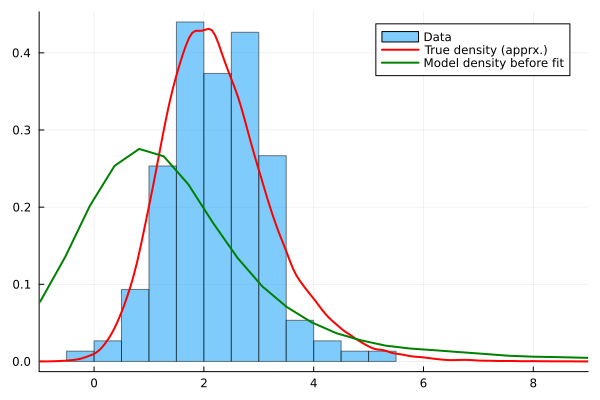

Random.seed!(123)


for i in 1:250
    
    gg = []
    
    for i in 1:10
        g = ForwardDiff.gradient(p->-particle_ll(f(p),Y), pars)
        push!(gg,g)
    end
    
    grads = mean(gg)
    
    pars.-=0.025.*grads
    
    
    if i%25 ==0
        println(particle_ll(f(pars),Y))
    end
end

-1.698369499604494
-1.5859668597849523
-1.4757647900932243
-1.3924143414512473
-1.3310941879731057
-1.2977140375800214
-1.2845731201786137
-1.2669498497241503
-1.2622906444844957
-1.2637100740914606

Ypostfit = rand(f(pars),50000)

histogram(Y,bins=20,normalize=true,alpha=0.5,label="Data",xlim=(-1,9),fmt=:png)
density!(Yfull,c=:red,lw=2, label="True density (apprx.)")
density!(Yprefit, c=:green,lw=2, label="Model density before fit")
density!(Ypostfit, c=:blue,lw=2, label="Fitted density")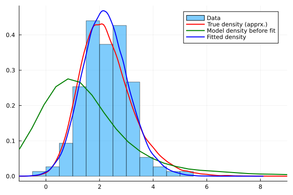

Stochastic volatility

\[X_t\sim\mathcal{N}(\alpha_h\cdot X_{t-1},\sigma_h^2);\quad -1<\alpha<1\] \[Y_t\sim\mathcal{N}(0,exp(X_t/4)^2)\]

\[X_0=0\] (could also be fitted/trained)

tanh(0.5)

0.46211715726000974

struct StochasticVolatilityModel
    alpha_h
    sigma_h
end
Flux.@functor StochasticVolatilityModel

StochasticVolatilityModel() = StochasticVolatilityModel(zeros(1,1).+atanh(0.5),zeros(1,1))

function Base.rand(m::StochasticVolatilityModel, T::Int, X_0=0.0)
    alpha_h = tanh(m.alpha_h[1])
    sigma_h = exp(m.sigma_h[1])
    
    X = [X_0]
    Y = []

    for t in 1:T
        X_t = randn() * sigma_h + alpha_h*X[end]
        Y_t = randn() * exp(X_t/4)
        
        push!(X,X_t)
        push!(Y,Y_t)
    end
        
    return X[2:end],Y
end

Base.rand(m::StochasticVolatilityModel) = rand(m,1)[1]

Specify model for a test case

\[X_t\sim\mathcal{N}(0.9\cdot X_{t-1},0.1^2);\quad -1<\alpha<1\] \[Y_t\sim\mathcal{N}(0,exp(X_t)^2)\]

Random.seed!(123)

m = StochasticVolatilityModel(atanh(0.95),0.1)

X,Y = rand(m,150)

plot(Y,fmt=:png)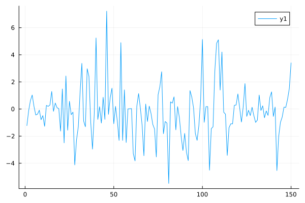

function particle_filter(m::StochasticVolatilityModel, y, M=1000)
    T = length(y)
    
    q0dist = Normal(0,3) #q_0(x)
    
    ps = rand(q0dist,(M,1))
    ws = [ones(M)./M]
    
    for t in 1:T
        qdists = Normal.(tanh(m.alpha_h[1]).*ps[:,t],exp(m.sigma_h[1]))
        ps_t = rand.(qdists)
        ps = hcat(ps,ps_t[:,:])
        odists = Normal.(0.0,exp.(ps_t./4))
        
        w_t = pdf.(odists,y[t])
        
        w_t = w_t./sum(w_t)
        
        a_t = rand(Categorical(w_t),M)
        ps = ps[a_t,:]
    end
        
    return ps[:,2:end]
end


function particle_filter_ll(m::StochasticVolatilityModel, y, M=1000)
    T = length(y)
    
    q0dist = Normal(0,3) #q_0(x)
    
    ps = rand(q0dist,(M,1))
    ws = [ones(M)./M]
    
    for t in 1:T
        qdists = Normal.(tanh(m.alpha_h[1]).*ps[:,t],exp(m.sigma_h[1]))
        ps_t = rand.(qdists)
        ps = hcat(ps,ps_t[:,:])
        odists = Normal.(0.0,exp.(ps_t./4))
        
        w_t = pdf.(odists,y[t])
        
        w_t = w_t./sum(w_t)
        
        a_t = rand(Categorical(w_t),M)
        ps = ps[a_t,:]
    end
        
    return mean(log.(mean(pdf.(Normal.(0.0,exp.(ps[:,2:end]./4)),transpose(y)),dims=1)))
end

particle_filter_ll (generic function with 2 methods)

Random.seed!(123)
ps_true = particle_filter(m,Y)

filter_mean_true = mean(exp.(ps_true./4),dims=1)[:]

plot(exp.(X./4),label="True Volatility",lw=2,fmt=:png)
plot!(filter_mean_true, label="Filter Mean True Model",lw=2)

ps_initial = particle_filter(StochasticVolatilityModel(),Y)


filter_mean_initial = mean(exp.(ps_initial./4),dims=1)[:]

plot!(filter_mean_initial, label="Filter Mean Initial Model",lw=2)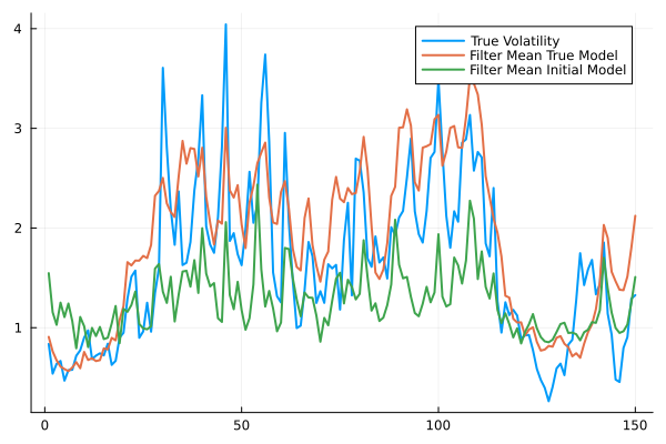

println(mean((X.-filter_mean_true).^2))

2.777623212726044

println(mean((X.-filter_mean_initial).^2))

4.1040430904059315

using FiniteDifferences

pars, f = Flux.destructure(StochasticVolatilityModel())

([0.5493061443340549, 0.0], Restructure(StochasticVolatilityModel, ..., 2))

Random.seed!(123)
for _ in 1:50
    gs = FiniteDifferences.grad(central_fdm(15,1),p->-mean([particle_filter_ll(f(p),Y,100) for _ in 1:5]),pars)[1]
    pars .-= 0.025.*gs
end

Random.seed!(123)

ps = particle_filter(f(pars),Y)

filter_mean_fitted = mean(exp.(ps./4),dims=1)[:]

plot(exp.(X./4),label="True Volatility",lw=2,fmt=:png)

plot!(filter_mean_true, label="Filter Mean True Model",lw=2)
plot!(filter_mean_fitted, label="Filter Mean Fitted Model",lw=2)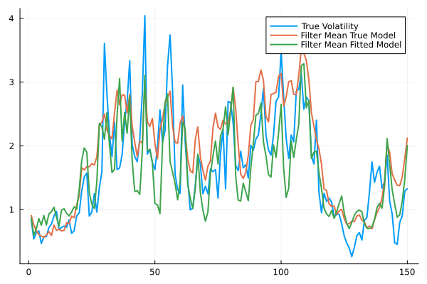

println(mean((X.-filter_mean_fitted).^2)) #much better than the initial model

3.174579327614477

pars #could probably be improved with longer training duration

2-element Vector{Float64}:
 0.7612290016866907
 0.4596682029518793